Ever since Windows’ inception, Microsoft Excel has been the go-to program for number-crunching, spreadsheets, invoices, and all the other things in life that you want organized into infinite grids of rows and columns.
But since the Cloud came to prominence, Google Sheets has become the program of choice for many people. It may not be as feature-rich as Excel, but there’s a lot more to it than first meets the eye.
Here are some tips and tricks for using Google Sheets which should ensure you get off to a smooth start.
Also read: 10 Google Sheets Add-ons You Should Consider Using
1. Import Data from Another Spreadsheet
You can easily set Google Sheets to dynamically import data from one of your spreadsheets to another. This is perfect if you want to show the sum of certain results in one spreadsheet, or if you want to move over a whole section of a table. Note that this isn’t the same as copying data because as you update the data in the original sheet, it will also update in the one you’re importing to.
The formula for this is known as ImportRange and looks something like this:
=IMPORTRANGE("1CwAtNKfeZ1IywYofZBVVsUZ9FJGB7uX6C0x3RMzW0VE","SheetName!A1:D200")The long cryptic code is the URL name of your spreadsheet, which you’ll find in the URL bar after “spreadsheets/d/”. Where it says “SheetName” above, you should replace with the name of the exact sheet you’re importing data from, then the bit after the exclamation mark represents the range of rows/columns you want to pull data from.
2. Freeze Rows and Columns
When you create a spreadsheet, in just about every case, you’ll want to have certain information displayed on your screen at all times. For example, if you’re keeping tabs on your freelance work, you’ll want to have header information like “Amount paid,” “Date of invoice” and “Website” constantly displayed even when you scroll down the page.
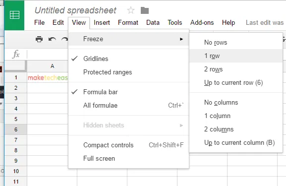
To do this, you’ll need to “Freeze” the row or column you want to always have on display. Just click “View -> Freeze,” then select the number of rows or columns you want to freeze. If you select a cell before clicking “View,” then you’ll get the option to freeze every row or column up to that cell.
3. Create Forms Using Google Sheets
A little known but brilliantly robust feature of Google Sheets is the option to create forms and questionnaires. Open a new Google Sheet, click “Tools -> Create a form,” and you’ll be taken to Google’s fancy Form-making app.
It’s pretty simple to use. You give the form a title and description, enter a question where it says “Untitled Question,” and then click “Multiple choice” if you want to change the format to where people can respond (multiple choice, checkboxes, dropdowns and so on).
At the top right of Forms, you’ll also see a trio of options that let you further customize the look of your questionnaire.

4. Insert Image Into a Cell
Before you get all clever and point out that inserting images into Google Sheets is just a matter of clicking “Insert -> Image,” well, not quite. If you use this method, then an image appears over the top of your spreadsheet rather than neatly placed into a cell.
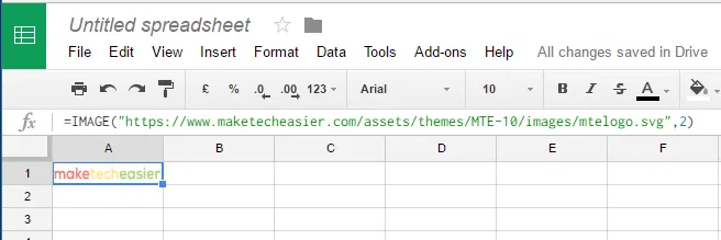
To insert an image straight into a cell, click the cell, then type =image("URL of the image you want to insert"). By default, the image will retain its aspect ratio while adapting to the cell size, but there are several variations you can make on the formula to get the image/cell the size you want.
=image("URL of the image",2)– reshapes the image to fit the existing cell size=image("URL of the image",3)– image keeps its original size without changing the cell size
5. Quickly Add Up Numbers
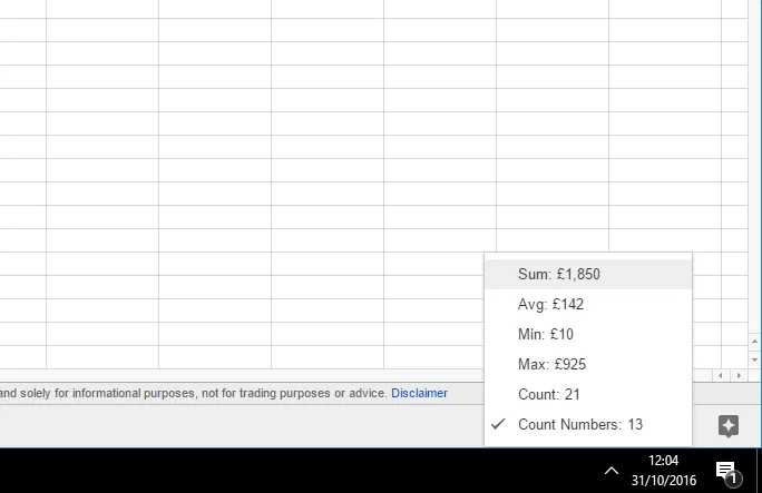
It’s a classic spreadsheet function and yet strangely easy to forget. Thankfully, Google Sheets makes things relatively easy for you. If you want to quickly add up the numbers in a row or column, simply highlight everything you want to calculate using left-mouse-click, and you’ll instantly see the sum of those numbers in the bottom-right corner of Google Sheets.
You can then click the sum at the bottom-right, and you’ll get a list of options to instead look at the average, smallest number, biggest number, and so on.
If you want to have a cell showing the sum total of a group of figures in a row or column, click the cell where you want the total to be displayed, then type =sum(A1:A13) where A1 and A13 are the cells where you want the numbers to be added up.
6. Conditional Formatting
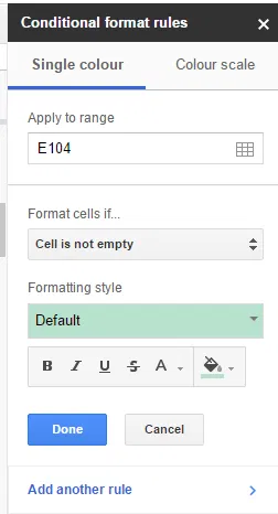
There’s nothing like a bit of color-coding to simplify all the Sheet data displayed in front of you. To set automatic rules for formatting and coloring cells, click “Format -> Conditional formatting.”
In a pane on the right, you’ll now see a bunch of “Conditional format rules.” Here you can get your spreadsheet to automatically color a cell red, for example, if it’s empty (a great way to instantly know if you need to chase anyone down for overdue payments), or paint cells containing a certain word a colour of your choice.
There are plenty of options here, so go wild! Your spreadsheet is your canvas.
7. Adding a Dropdown option to your cell
Let’s say that you want to limit the content of a cell to only two (or more) values. The best way to implement this is to add a Dropdown option. To do that you will have to create a new Sheet to hold the option values.
1. Create a new Sheet by clicking the “+” icon on the bottom toolbar.

2. In the new sheet enter your option values in the first column.
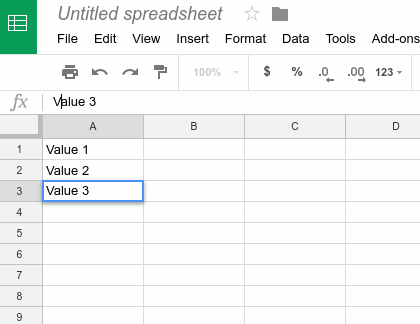
3. Back to the first Sheet (or the sheet that you are working on), select the cell where you want to insert the dropdown.
4. Right click on it and select “Data Validation” (at the very end of the context menu).
5. In the “Criteria” field, select “List from a range” and select the Sheet, columns and cell in the “Data” field. Check the option “Show dropdown list in cell.”
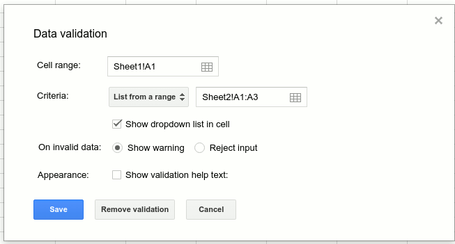
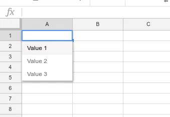
6. Click OK. You should now see the Dropdown field where you can limit the content of the cell to a specific range of value.
The ideal situation to be in with a spreadsheet is to have a whole bunch of rules that automate things like colour-coding and calculations so that you can work as quickly and efficiently as possible. Hopefully these five tips will help you achieve that, make the information contained therein a whole lot clearer and spice up the sometimes sterile process of managing a spreadsheet.
Image credit: Close-up Of A Person’s Hand Typing On Laptop Over Wooden Desk by 123RF


Comments on " How to Use Google Sheets: Key Tips to Get You Started" :